Super fast color transfer between images

By Adrian Rosebrock on June 30, 2014 in Image Processing, Tutorials

About a month ago, I spent a morning down at the beach, walking along the sand, letting the crisp, cold water lap against my feet. It was tranquil, relaxing. I then took out my iPhone and snapped a few photos of the ocean and clouds passing by. You know, something to remember the moment by. Because I knew that as soon as I got back to the office, that my nose was going back on the grindstone.

Back at home, I imported my photos to my laptop and thought, hey, there must be a way to take this picture of the beach that I took during the mid-morning and make it look like it was taken at dusk.

And since I’m a computer vision scientist, I certainly wasn’t going to resort to Photoshop.

No, this had to be a hand engineered algorithm that could take two arbitrary images, a source and a target, and then transfer the color space from the source image to the target image.

A couple weeks ago I was browsing reddit and I came across a post on how to transfer colors between two images. The authors’ implementation used a histogram based method, which aimed to balance between three “types” of bins: equal, excess, and deficit.

The approach obtained good results — but at the expense of speed. Using this algorithm would require you to perform a lookup for each and every pixel in the source image, which will become extremely expensive as the image grows in size. And while you can certainly speed the process up using a little NumPy magic you can do better.

Much, much better in fact.

What if I told you that you could create a color transfer algorithm that uses nothing but the mean and standard deviation of the image channels.

That’s it. No complicated code. No computing histograms. Just simple statistics.

And by the way…this method can handle even gigantic images with ease.

Interested?

Read on.

You can also download the code via GitHub or install via PyPI (assuming that you already have OpenCV installed).

The Color Transfer Algorithm

My implementation of color transfer is (loosely) based on Color Transfer between Images by Reinhard et al, 2001.

In this paper, Reinhard and colleagues demonstrate that by utilizing the L*a*b* color space and the mean and standard deviation of each L*, a*, and b* channel, respectively, that the color can be transferred between two images.

The algorithm goes like this:

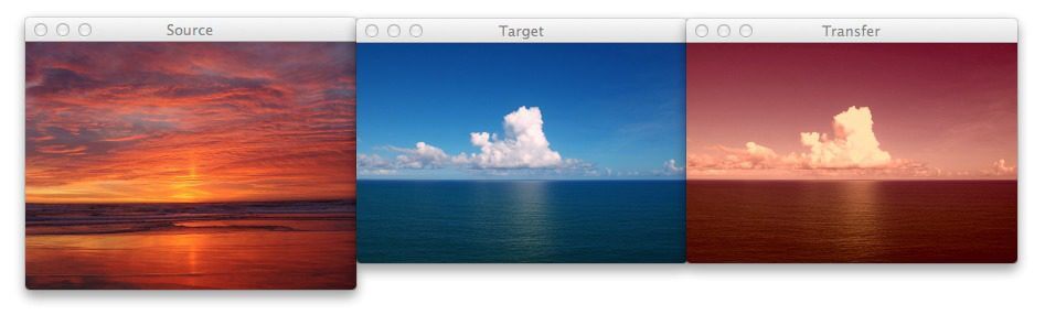
Step 1: Input a source and a target image. The source image contains the color space that you want your target image to mimic. In the figure at the top of this page, the sunset image on the left is my source, the middle image is my target, and the image on the right is the color space of the source applied to the target.
Step 2: Convert both the source and the target image to the L*a*b* color space. The L*a*b* color space models perceptual uniformity, where a small change in an amount of color value should also produce a relatively equal change in color importance. The L*a*b* color space does a substantially better job mimicking how humans interpret color than the standard RGB color space, and as you’ll see, works very well for color transfer.
Step 3: Split the channels for both the source and target.
Step 4: Compute the mean and standard deviation of each of the L*a*b* channels for the source and target images.
Step 5: Subtract the mean of the L*a*b* channels of the target image from target channels.
Step 6: Scale the target channels by the ratio of the standard deviation of the target divided by the standard deviation of the source, multiplied by the target channels.
Step 7: Add in the means of the L*a*b* channels for the source.
Step 8: Clip any values that fall outside the range [0, 255]. (Note: This step is not part of the original paper. I have added it due to how OpenCV handles color space conversions. If you were to implement this algorithm in a different language/library, you would either have to perform the color space conversion yourself, or understand how the library doing the conversion is working).
Step 9: Merge the channels back together.
Step 10: Convert back to the RGB color space from the L*a*b* space.

I know that seems like a lot of steps, but it’s really not, especially given how simple this algorithm is to implement when using Python, NumPy, and OpenCV.

If it seems a bit complex right now, don’t worry. Keep reading and I’ll explain the code that powers the algorithm.

Requirements

I’ll assume that you have Python, OpenCV (with Python bindings), and NumPy installed on your system.

If anyone wants to help me out by creating a requirements.txt file in the GitHub repo, that would be super awesome.

Install

Assuming that you already have OpenCV (with Python bindings) and NumPy installed, the easiest way to install is use to use pip:

$ pip install color_transfer

1	$ pip install color_transfer

The Code Explained

I have created a PyPI package that you can use to perform color transfer between your own images. The code is also available on GitHub.

Anyway, let’s roll up our sleeves, get our hands dirty, and see what’s going on under the hood of the color_transfer package:

# import the necessary packages
import numpy as np
import cv2

def color_transfer(source, target):
	# convert the images from the RGB to L*ab* color space, being
	# sure to utilizing the floating point data type (note: OpenCV
	# expects floats to be 32-bit, so use that instead of 64-bit)
	source = cv2.cvtColor(source, cv2.COLOR_BGR2LAB).astype("float32")
	target = cv2.cvtColor(target, cv2.COLOR_BGR2LAB).astype("float32")

# import the necessary packages

import numpy as np

import cv2

def color_transfer(source, target):

# convert the images from the RGB to L*ab* color space, being

# sure to utilizing the floating point data type (note: OpenCV

# expects floats to be 32-bit, so use that instead of 64-bit)

source = cv2.cvtColor(source, cv2.COLOR_BGR2LAB).astype("float32")

target = cv2.cvtColor(target, cv2.COLOR_BGR2LAB).astype("float32")

Lines 2 and 3 import the packages that we’ll need. We’ll use NumPy for numerical processing and cv2 for our OpenCV bindings.

From there, we define our color_transfer function on Line 5. This function performs the actual transfer of color from the source image (the first argument) to the target image (the second argument).

The algorithm detailed by Reinhard et al. indicates that the L*a*b* color space should be utilized rather than the standard RGB. To handle this, we convert both the source and the target image to the L*a*b* color space on Lines 9 and 10 (Steps 1 and 2).

OpenCV represents images as multi-dimensional NumPy arrays, but defaults to the uint8 datatype. This is fine for most cases, but when performing the color transfer we could potentially have negative and decimal values, thus we need to utilize the floating point data type.

Now, let’s start performing the actual color transfer:

# import the necessary packages
import numpy as np
import cv2

def color_transfer(source, target):
	# convert the images from the RGB to L*ab* color space, being
	# sure to utilizing the floating point data type (note: OpenCV
	# expects floats to be 32-bit, so use that instead of 64-bit)
	source = cv2.cvtColor(source, cv2.COLOR_BGR2LAB).astype("float32")
	target = cv2.cvtColor(target, cv2.COLOR_BGR2LAB).astype("float32")

	# compute color statistics for the source and target images
	(lMeanSrc, lStdSrc, aMeanSrc, aStdSrc, bMeanSrc, bStdSrc) = image_stats(source)
	(lMeanTar, lStdTar, aMeanTar, aStdTar, bMeanTar, bStdTar) = image_stats(target)

	# subtract the means from the target image
	(l, a, b) = cv2.split(target)
	l -= lMeanTar
	a -= aMeanTar
	b -= bMeanTar

	# scale by the standard deviations
	l = (lStdTar / lStdSrc) * l
	a = (aStdTar / aStdSrc) * a
	b = (bStdTar / bStdSrc) * b

	# add in the source mean
	l += lMeanSrc
	a += aMeanSrc
	b += bMeanSrc

	# clip the pixel intensities to [0, 255] if they fall outside
	# this range
	l = np.clip(l, 0, 255)
	a = np.clip(a, 0, 255)
	b = np.clip(b, 0, 255)

	# merge the channels together and convert back to the RGB color
	# space, being sure to utilize the 8-bit unsigned integer data
	# type
	transfer = cv2.merge([l, a, b])
	transfer = cv2.cvtColor(transfer.astype("uint8"), cv2.COLOR_LAB2BGR)
	
	# return the color transferred image
	return transfer

# compute color statistics for the source and target images

(lMeanSrc, lStdSrc, aMeanSrc, aStdSrc, bMeanSrc, bStdSrc) = image_stats(source)

(lMeanTar, lStdTar, aMeanTar, aStdTar, bMeanTar, bStdTar) = image_stats(target)

# subtract the means from the target image

(l, a, b) = cv2.split(target)

l -= lMeanTar

a -= aMeanTar

b -= bMeanTar

# scale by the standard deviations

l = (lStdTar / lStdSrc) * l

a = (aStdTar / aStdSrc) * a

b = (bStdTar / bStdSrc) * b

# add in the source mean

l += lMeanSrc

a += aMeanSrc

b += bMeanSrc

# clip the pixel intensities to [0, 255] if they fall outside

# this range

l = np.clip(l, 0, 255)

a = np.clip(a, 0, 255)

b = np.clip(b, 0, 255)

# merge the channels together and convert back to the RGB color

# space, being sure to utilize the 8-bit unsigned integer data

# type

transfer = cv2.merge([l, a, b])

transfer = cv2.cvtColor(transfer.astype("uint8"), cv2.COLOR_LAB2BGR)

# return the color transferred image

return transfer

Lines 13 and 14 make calls to the image_stats function, which I’ll discuss in detail in a few paragraphs. But for the time being, know that this function simply computes the mean and standard deviation of the pixel intensities for each of the L*, a*, and b* channels, respectively (Steps 3 and 4).

Now that we have the mean and standard deviation for each of the L*a*b* channels for both the source and target images, we can now perform the color transfer.

On Lines 17-20, we split the target image into the L*, a*, and b* components and subtract their respective means (Step 5).

From there, we perform Step 6 on Lines 23-25 by scaling by the ratio of the target standard deviation, divided by the standard deviation of the source image.

Then, we can apply Step 7, by adding in the mean of the source channels on Lines 28-30.

Step 8 is handled on Lines 34-36 where we clip values that fall outside the range [0, 255] (in the OpenCV implementation of the L*a*b* color space, the values are scaled to the range [0, 255], although that is not part of the original L*a*b* specification).

Finally, we perform Step 9 and Step 10 on Lines 41 and 42 by merging the scaled L*a*b* channels back together, and finally converting back to the original RGB color space.

Lastly, we return the color transferred image on Line 45.

Let’s take a quick look at the image_stats function to make this code explanation complete:

# import the necessary packages
import numpy as np
import cv2

def color_transfer(source, target):
	# convert the images from the RGB to L*ab* color space, being
	# sure to utilizing the floating point data type (note: OpenCV
	# expects floats to be 32-bit, so use that instead of 64-bit)
	source = cv2.cvtColor(source, cv2.COLOR_BGR2LAB).astype("float32")
	target = cv2.cvtColor(target, cv2.COLOR_BGR2LAB).astype("float32")

	# compute color statistics for the source and target images
	(lMeanSrc, lStdSrc, aMeanSrc, aStdSrc, bMeanSrc, bStdSrc) = image_stats(source)
	(lMeanTar, lStdTar, aMeanTar, aStdTar, bMeanTar, bStdTar) = image_stats(target)

	# subtract the means from the target image
	(l, a, b) = cv2.split(target)
	l -= lMeanTar
	a -= aMeanTar
	b -= bMeanTar

	# scale by the standard deviations
	l = (lStdTar / lStdSrc) * l
	a = (aStdTar / aStdSrc) * a
	b = (bStdTar / bStdSrc) * b

	# add in the source mean
	l += lMeanSrc
	a += aMeanSrc
	b += bMeanSrc

	# clip the pixel intensities to [0, 255] if they fall outside
	# this range
	l = np.clip(l, 0, 255)
	a = np.clip(a, 0, 255)
	b = np.clip(b, 0, 255)

	# merge the channels together and convert back to the RGB color
	# space, being sure to utilize the 8-bit unsigned integer data
	# type
	transfer = cv2.merge([l, a, b])
	transfer = cv2.cvtColor(transfer.astype("uint8"), cv2.COLOR_LAB2BGR)
	
	# return the color transferred image
	return transfer

def image_stats(image):
	# compute the mean and standard deviation of each channel
	(l, a, b) = cv2.split(image)
	(lMean, lStd) = (l.mean(), l.std())
	(aMean, aStd) = (a.mean(), a.std())
	(bMean, bStd) = (b.mean(), b.std())

	# return the color statistics
	return (lMean, lStd, aMean, aStd, bMean, bStd)

def image_stats(image):

# compute the mean and standard deviation of each channel

(l, a, b) = cv2.split(image)

(lMean, lStd) = (l.mean(), l.std())

(aMean, aStd) = (a.mean(), a.std())

(bMean, bStd) = (b.mean(), b.std())

# return the color statistics

return (lMean, lStd, aMean, aStd, bMean, bStd)

Here we define the image_stats function, which accepts a single argument: the image that we want to compute statistics on.

We make the assumption that the image is already in the L*a*b* color space, prior to calling cv2.split on Line 49 to break our image into its respective channels.

From there, Lines 50-52 handle computing the mean and standard deviation of each of the channels.

Finally, a tuple of mean and standard deviations for each of the channels are returned on Line 55.

Examples

To grab the example.py file and run examples, just grab the code from the GitHub project page.

You have already seen the beach example at the top of this post, but let’s take another look:

$ python example.py --source images/ocean_sunset.jpg --target images/ocean_day.jpg

1	$ python example.py --source images/ocean_sunset.jpg --target images/ocean_day.jpg

After executing this script, you should see the following result:

Super Fast Color Transfer between Images

Figure 1: The image on the left is the source, the middle image is the target, and the right is the output image after applying the color transfer from the source to the target. Notice how a nice sunset effect is created in the output image.

Notice how the oranges and reds of the sunset photo has been transferred over to the photo of the ocean during the day.

Awesome. But let’s try something different:

$ python example.py --source images/woods.jpg --target images/storm.jpg

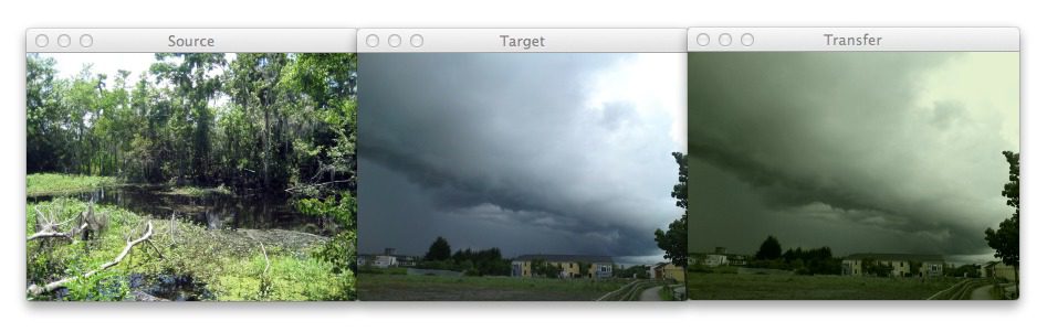
1	$ python example.py --source images/woods.jpg --target images/storm.jpg

Figure 2: Using color transfer to make storm clouds look much more ominous using the green foliage of a forest scene.

Here you can see that on the left we have a photo of a wooded area — mostly lots of green related to vegetation and dark browns related to the bark of the trees.

And then in the middle we have an ominous looking thundercloud — but let’s make it more ominous!

If you have ever experienced a severe thunderstorm or a tornado, you have probably noticed that the sky becomes an eerie shade of green prior to the storm.

As you can see on the right, we have successfully mimicked this ominous green sky by mapping the color space of the wooded area to our clouds.

Pretty cool, right?

One more example:

$ python example.py --source images/autumn.jpg --target images/fallingwater.jpg

1	$ python example.py --source images/autumn.jpg --target images/fallingwater.jpg

Figure 3: Using color transfer between images to create an autumn style effect on the output image.

Here I am combining two of my favorite things: Autumn leaves (left) and mid-century modern architecture, in this case, Frank Lloyd Wright’s Fallingwater (middle).

The middle photo of Fallingwater displays some stunning mid-century architecture, but what if I wanted to give it an “autumn” style effect?

You guessed it — transfer the color space of the autumn image to Fallingwater! As you can see on the right, the results are pretty awesome.

Ways to Improve the Algorithm

While the Reinhard et al. algorithm is extremely fast, there is one particular downside — it relies on global color statistics, and thus large regions with similar pixel intensities values can dramatically influence the mean (and thus the overall color transfer).

To remedy this problem, we can look at two solutions:

Option 1: Compute the mean and standard deviation of the source image in a smaller region of interest (ROI) that you would like to mimic the color of, rather than using the entire image. Taking this approach will make your mean and standard deviation better represent the color space you want to use.

Option 2: The second approach is to apply k-means to both of the images. You can cluster on the pixel intensities of each image in the L*a*b* color space and then determine the centroids between the two images that are most similar using the Euclidean distance. Then, compute your statistics within each of these regions only. Again, this will give your mean and standard deviation a more “local” effect and will help mitigate the overrepresentation problem of global statistics. Of course, the downside is that this approach is substantially slower, since you have now added in an expensive clustering step.

Summary

In this post I showed you how to perform a super fast color transfer between images using Python and OpenCV.

I then provided an implementation based (loosely) on the Reinhard et al. paper.

Unlike histogram based color transfer methods which require computing the CDF of each channel and then constructing a Lookup Table (LUT), this method relies strictly on the mean and standard deviation of the pixel intensities in the L*a*b* color space, making it extremely efficient and capable of processing very large images quickly.

If you are looking to improve the results of this algorithm, consider applying k-means clustering on both the source and target images, matching the regions with similar centroids, and then performing color transfer within each individual region. Doing this will use local color statistics rather than global statistics and thus make the color transfer more visually appealing.

Code Available on GitHub

Looking for the source code to this post? Just head over to the GitHub project page!

Learn the Basics of Computer Vision in a Single Weekend

If you’re interested in learning the basics of computer vision, but don’t know where to start, you should definitely check out my new eBook, Practical Python and OpenCV.

In this book I cover the basics of computer vision and image processing…and I can teach you in a single weekend!

I know, it sounds too good to be true.

But I promise you, this book is your guaranteed quick-start guide to learning the fundamentals of computer vision. After reading this book you will be well on your way to becoming an OpenCV guru!

So if you’re looking to learn the basics of OpenCV, definitely check out my book. You won’t be disappointed.

color space, color transfer, image processing, lab, reinhard et al, rgb

Announcing “Case Studies: Solving real world problems with computer vision”

Color Quantization with OpenCV using K-Means Clustering

37 Responses to Super fast color transfer between images

copain July 1, 2014 at 10:41 am #

G’MIC has a filter named Transfer Color : https://secure.flickr.com/groups/gmic/discuss/72157625453465326/. Even if you’re not a photoshop guy, I believe G’MIC is very interesting.

Reply
- Adrian Rosebrock July 2, 2014 at 5:38 am #
  
  Wow, thanks for the link. This is some really great stuff.
  
  Reply
damianfral July 20, 2014 at 7:18 pm #

I’ve done something similar (almost a clone of your program) but using YCbCr color space: https://github.com/damianfral/colortransfer. The results are pretty similar, but I see “my version a little bit more saturated.

The YCbCr color spaces, unlike Lab, is linear, so transforming RGB to YCbCr (and viceversa) has less complexity than transforming from RGB to Lab, which could give us a performance improvement.

PS: Thanks for these articles, they are really interesting. 🙂

Reply
- Adrian Rosebrock July 21, 2014 at 6:07 am #
  
  Very cool, thanks for porting it over to Haskell. And I’m glad you like the articles!
  
  Reply
rb August 27, 2014 at 10:02 am #

Hi Thanks for the article, very clear & useful.

But I think the scaling is inverted — shouldn’t lines 23-25 be:

l = (lStdSrc / lStdTar) * l
a = (aStdSrc / aStdTar) * a
b = (bStdSrc / bStdTar) * b

Also, any reason not to use *= ?

l *= lStdSrc / lStdTar
a *= aStdSrc / aStdTar
b *= bStdSrc / bStdTar

Thanks again

Reply
- Adrian Rosebrock August 27, 2014 at 11:43 am #
  
  Hi rb, thanks for the comment.
  
  Take a look at the original color transfer paper by Reinhard et al. On Page 3 you’ll see Equation 11. This is the correct equation to apply, so the scaling is not inverted, although I can see why it could see confusing.
  
  Also, *= could be used, but again, I kept to the form of Equation 11 just for the sake of simplicity.
  
  Reply
  - Nrupatunga October 29, 2014 at 1:31 pm #
    
    Hi Adrian,
    As rb mentioned, scaling should be as follows right?
    
    l = (lStdSrc / lStdTar) * l]
    a = (aStdSrc / aStdTar) * a
    b = (bStdSrc / bStdTar) * b
    
    This is because the final transformed image(target) should have the statistical values(mean and standard deviation) of source image right?
    
    Please correct me if I am wrong.
    
    Reply
    - Adrian Rosebrock November 4, 2014 at 6:50 am #
      
      The scaling is actually correct — I provided an explanation for why in the comment reply to Rb above.
      
      Furthermore, take a look at this closed issue on GitHub for a detailed explanation. Specifically, take a look at Equation 11 of this paper.
      
      Reply
  - AP January 10, 2015 at 8:45 am #
    
    Hey Adrian. I agree with previous commenters that scaling should be inverted.
    The eq. 11 from original paper is correct, but your definitions of source and target images are not same as in the paper.
    Your method color_transfer(source, target) modifies target image using statistics from source image (at least it does correctly for mean value).
    But if you read paper carefully (e.g. see description of picture 2), they use statistics from target image and apply it to source image.
    You have good results because mean value for a, b channels have major contribution in color transfer.
    
    Reply
    - Adrian Rosebrock January 10, 2015 at 12:37 pm #
      
      So I took a look at the description of Figure 2 which states: “Color correction in different color spaces. From top to bottom, the original source and target images”, followed by the corrected images …”. Based off this wording (especially since the “source” image is listed first) and Equation 11, I still think the scaling is correct. If only I could get in touch with Reinhard et al. to resolve the issue!
      
      Reply
      - AP January 10, 2015 at 2:16 pm #
        
        So, you can see from pic 2, that corrected images are source image with target image colors applied, but not target image with colors from source image as in your code.
      - Adrian Rosebrock January 10, 2015 at 5:10 pm #
        
        That’s just for one example though, and it doesn’t follow the intuition of Equation 11. I’ll continue to give this some thought. When I reversed the standard deviations the result image ended up looking very over-saturated. This comment thread could probably turn into a good follow-up blog post.
NickShargan December 1, 2014 at 2:20 pm #

Wow, it works!

Reply
zizek February 8, 2015 at 9:35 am #

I thought that your method woudn’t much faster than using LUT with CDF histogram. Because your method have to re-build ‘Lab’ color model and calculate means and stds through every pixels in each channels. Did you compare the computational time of two methods?

Reply
- Adrian Rosebrock February 8, 2015 at 12:47 pm #
  
  I don’t have any benchmarks, but thanks for suggesting that. I will look into creating some. Furthermore, calculating the mean and standard deviation for each channel is extremely fast due to the vectorized operations of NumPy under the hood.
  
  Reply
Darwin April 13, 2015 at 12:01 pm #

Why OpenCV does not implement any colorization algorithm ?

Reply
- Adrian Rosebrock April 13, 2015 at 1:34 pm #
  
  Hi Darwin, what do you mean by “colorization”?
  
  Reply
Kewal January 18, 2016 at 11:24 am #

When applying k-means clustering to both source and target images, how to find similar centroids?

Reply
- Adrian Rosebrock January 18, 2016 at 3:17 pm #
  
  Simply compute the Euclidean distance between the centroids. The smaller the distance, the more “similar” the clusters are.
  
  Reply
Rastislav Zima February 3, 2016 at 2:55 am #

Hi Adrian, have you tried to apply your algorithm to the pictures from the document http://www.cs.tau.ac.il/~turkel/imagepapers/ColorTransfer.pdf ? It seems to me that the example pictures you have used are not equalised exactly in the same way as in this document – the colors are there but the resulting contrast of the pictures seems not to be the same as in the source, but it’s hard to judge without using same examples.

Reply
- Adrian Rosebrock February 4, 2016 at 9:21 am #
  
  Indeed, that is the paper I used as inspiration for that post. It’s hard to validate if the results are 100% correct or not without having access to the raw images that the authors used.
  
  Reply
gustavo February 6, 2016 at 9:46 am #

Good technique. But i´m not being able to port to other languages. I don´t know what the clip does !

I mean, it clips values to 255, but……Lab value are not from 0 to 255 !!! When converting RGB to Lab the values of Lab are from 0 to 100 !

There are maximum limits for Lab but they are not to be cliped at 255. If you consider using the white reference observer, you will see that for D65 the whitespace limits used during the convertion from XYz to Lab are:

WHITE_SPACE_D65_X2 95.047
WHITE_SPACE_D65_Y2 100
WHITE_SPACE_D65_Z2 108.883

I´m confused about the python code (since i don´t know python). Can you build a example using C Apis ? (32 Bits plain C, i mean..no mfc, or .net)

Thanks, in advance

Reply
- Adrian Rosebrock February 6, 2016 at 9:53 am #
  
  If you’re using OpenCV for C++, then the cv2.cvtColor function will automatically handle the color space conversion and (should) but the color values in the range [0, 255]. You can confirm this for yourself by examining pixel values after the color space conversion.
  
  Reply
gustavo trigueiros February 8, 2016 at 1:31 pm #

Hi Adrian. I finally make it work 🙂 I was making some mistakes on the color conversion algorithms, but now, it seems to working as expected. I´ll clean up the code and make further tests and post it here to you see. I made some small changes on the way the Standard Deviations for Luma, afactor, bfactor are being collected/ued, but it is working extremelly fast. One of the modifications i made was to avoid computing when the pixels under analysis have the same Luma or aFact/bFact. On those cases, it means that the pixels are the same, so don´t need to compute the STD operations.
On this way, it avoids to you use as source and target the same image. The result without that was that the image coloring was changing bevcause it was computing the STD operations. So, one update i made was to simply let it unchanged when the values of both pixels are the same.
So, it will only use the STD on values that are different from source and target.
If image1 have Luma different then Image2 it will use it the STD operations
If image1 have AFactor different then Image2 it will use it the STD operations
If image1 have BFactor different then Image2 it will use it the STD operations

I´m amazed about the results, and deeply impressed.Congrats !

Reply
- Adrian Rosebrock February 8, 2016 at 3:44 pm #
  
  Thanks for sharing Gustavo!
  
  Reply
gustavo trigueiros February 8, 2016 at 10:02 pm #

You´re welcome 🙂

The algo works like a charm, and the scaling factor can work on different ways to determine how saturated (contrasted) the image can result.

For example, forcing the scaling factor for Luma, A and B result in smaller then 1 (when STDSrc < StdTarget, resuts STDSrc/StdTarget STDTarget) improves the overall brightness and contrast of the image, but…if the target image have areas where it was already bright, it will loose it´s details due to the over saturation of the colors. Like on the image below

http://i66.tinypic.com/scxnow.jpg

This variances of contrast according to the scaling factor are good if we want to built a function that do the color transferring and have as one or more parameters a contrast enhancer from where the user can choose the amount of contrast to be used. I mean, how the results will be displayed, if oversaturated or not.

Also, if you use Scaling Facot for luma be smaller then 1 and A and B be bigger then 1, you have a more pleasant look of the image as seeing here

http://i68.tinypic.com/j90s93.jpg

I´m still making further tests and trying to optimize the function but so far, i´m very impressed with the results.

And also, it can be used to transfer from colored to grayscale images, although the grayscaled image won´t turn onto a full colored one, it may have a beautifull tone depending of the colors of the source.

Btw…thinking in that subject, perhaps it is possible to color a grayscale image biased on the colors of the source ? The algorithm maybe used to do that, i suppose comparing the std of all the channels of the coloured image with the one from the grayscale and choosing the one that best fits with the target (the grayscale one). Once it is chosen, the simply trnasfer the chroma from a/b from the source to the gray image ?

Reply
ahmed ramzy April 8, 2016 at 11:47 pm #

Thanks for such a tutorial , i liked it alot (Y)

I’ll share my results with my friends,and i am asking if i can also share this link with them ?

Reply
- Adrian Rosebrock April 13, 2016 at 7:16 pm #
  
  Sure, by all means, please share the PyImageSearch blog with your friends!
  
  Reply
Indra May 29, 2017 at 3:31 pm #

Hi Adrian,

Thanks for the blog post with such good stuff. But I have doubt in the suggestion you gave when using KMeans clustering. What is the reason behind finding similar centroids ? Can you give an intuition behind this ?

Reply
- Adrian Rosebrock May 31, 2017 at 1:18 pm #
  
  The general idea is that by finding similar color centroids you could potentially achieve a more aesthetically pleasing color transfer.
  
  Reply
  - Saumya July 17, 2017 at 1:46 am #
    
    are you referring to position wise transfer using Kmeans clustering?
    
    Reply
Hansa July 25, 2017 at 2:13 pm #

What the result if target image is grayscale image

Reply
- Adrian Rosebrock July 28, 2017 at 10:04 am #
  
  Are you trying to transfer the color of a color image to a grayscale image? If so, that won’t work. You’ll want to research methods on colorizing grayscale images. Deep learning has had great success here.
  
  Reply
Jon November 21, 2017 at 6:27 am #

Hey Adrian, first of all – thank you for the great post and making the transfer method from the paper so easily accessible. Really great stuff!
I’m fairly new to image processing but I gave this a shot, got stuck and was wondering if you had any ideas: The main problem I’m seeing with my implementation of the suggested k-means approach is that when statistics are computed in similar regions the localized transfers result in banding along the cluster boundaries. Interpolating over the boundaries feels a bit like a hack and produces unstable results. Do you have any pointers to how a localization of the transfer could be smoothed?

Reply
- Adrian Rosebrock November 21, 2017 at 1:21 pm #
  
  Hey Jon — indeed, you have stumbled on to the biggest problem with the k-means approach. Color transfer isn’t my particular area of expertise (although I find it super interesting) so I’m not sure what the best method would be. I would consult this paper which I know the locality-preserving color transfer approach in more detail.
  
  Reply
  - Jon November 21, 2017 at 3:11 pm #
    
    Exactly what I’ve been looking for! Thanks again.
    
    Reply
m February 18, 2018 at 9:49 am #

Hi, I want to run this code for c# and using opencv
But with the difference that instead of the colors of the source image, the different colors I give myself apply to the target image.
Can anyone help me?
My email :

Reply

Navigation