Gradient Descent with Python

Nearly all of deep learning is powered by one very important algorithm: Stochastic Gradient Descent (SGD).

— Goodfellow, Bengio, and Courville (2016)

At this point, we have a strong understanding of the concept of parameterized learning. We previously discussed the concept of parameterized learning and how this type of learning enables us to define a scoring function that maps our input data to output class labels.

This scoring function is defined in terms of two important parameters; specifically, our weight matrix W and our bias vector b. Our scoring function accepts these parameters as inputs and returns a prediction for each input data point x_i.

We have also discussed two common loss functions: Multi-class SVM loss and cross-entropy loss. Loss functions, at the most basic level, are used to quantify how “good” or “bad” a given predictor (i.e., a set of parameters) is at classifying the input data points in our data.

Given these building blocks, we can now move on to the most important aspect of machine learning, neural networks, and deep learning — optimization. Optimization algorithms are the engines that power neural networks and enable them to learn patterns from data. Throughout this discussion, we’ve learned that obtaining a high accuracy classifier is dependent on finding a set of weights W and b such that our data points are correctly classified.

But how do we go about finding and obtaining a weight matrix W and bias vector b that obtains high classification accuracy? Do we randomly initialize them, evaluate, and repeat over and over again, hoping that at some point we land on a set of parameters that obtains reasonable classification? We could — but given that modern deep learning networks have parameters that number in the tens of millions, it may take us a long time to blindly stumble upon a reasonable set of parameters.

Instead of relying on pure randomness, we need to define an optimization algorithm that allows us to literally improve W and b. In this lesson, we’ll be looking at the most common algorithm used to train neural networks and deep learning models — gradient descent. Gradient descent has many variants (which we’ll also touch on), but, in each case, the idea is the same: iteratively evaluate your parameters, compute your loss, then take a small step in the direction that will minimize your loss.

Gradient Descent with Python

The gradient descent algorithm has two primary flavors:

1. The standard “vanilla” implementation.
2. The optimized “stochastic” version that is more commonly used.

In this lesson, we’ll be reviewing the basic vanilla implementation to form a baseline for our understanding. After we understand the basics of gradient descent, we’ll move on to the stochastic version. We’ll then review some of the “bells and whistles” that we can add on to gradient descent, including momentum, and Nesterov acceleration.

The Loss Landscape and Optimization Surface

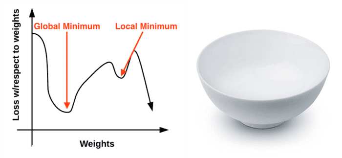
The gradient descent method is an iterative optimization algorithm that operates over a loss landscape (also called an optimization surface). The canonical gradient descent example is to visualize our weights along the x-axis and then the loss for a given set of weights along the y-axis (Figure 1, left):

As we can see, our loss landscape has many peaks and valleys based on which values our parameters take on. Each peak is a local maximum that represents very high regions of loss — the local maximum with the largest loss across the entire loss landscape is the global maximum. Similarly, we also have local minimum which represents many small regions of loss.

The local minimum with the smallest loss across the loss landscape is our global minimum. In an ideal world, we would like to find this global minimum, ensuring our parameters take on the most optimal possible values.

So that raises the question: “If we want to reach a global minimum, why not just directly jump to it? It’s clearly visible on the plot?”

Therein lies the problem — the loss landscape is invisible to us. We don’t actually know what it looks like. If we’re an optimization algorithm, we would be blindly placed somewhere on the plot, having no idea what the landscape in front of us looks like, and we would have to navigate our way to a loss minimum without accidentally climbing to the top of a local maximum.

Personally, I’ve never liked this visualization of the loss landscape — it’s too simple, and it often leads readers to think that gradient descent (and its variants) will eventually find either a local or global minimum. This statement isn’t true, especially for complex problems — and I’ll explain why later. Instead, let’s look at a different visualization of the loss landscape that I believe does a better job depicting the problem. Here we have a bowl, similar to the one you may eat cereal or soup out of (Figure 1, right).

The surface of our bowl is the loss landscape, which is a plot of the loss function. The difference between our loss landscape and your cereal bowl is that your cereal bowl only exists in three dimensions, while your loss landscape exists in many dimensions, perhaps tens, hundreds, or thousands of dimensions.

Each position along the surface of the bowl corresponds to a particular loss value given a set of parameters W (weight matrix) and b (bias vector). Our goal is to try different values of W and b, evaluate their loss, and then take a step toward more optimal values that (ideally) have lower loss.

The “Gradient” in Gradient Descent

To make our explanation of gradient descent a little more intuitive, let’s pretend that we have a robot — let’s name him Chad (Figure 2, left). When performing gradient descent, we randomly drop Chad somewhere on our loss landscape (Figure 2, right).

It’s now Chad’s job to navigate to the bottom of the basin (where there is minimum loss). Seems easy enough right? All Chad has to do is orient himself such that he’s facing “downhill” and ride the slope until he reaches the bottom of the bowl.

But here’s the problem: Chad isn’t a very smart robot. Chad has only one sensor — this sensor allows him to take his parameters W and b and then compute a loss function L. Therefore, Chad is able to compute his relative position on the loss landscape, but he has absolutely no idea in which direction he should take a step to move himself closer to the bottom of the basin.

What is Chad to do? The answer is to apply gradient descent. All Chad needs to do is follow the slope of the gradient W. We can compute the gradient W across all dimensions using the following equation:

(1)

In dimensions > 1, our gradient becomes a vector of partial derivatives. The problem with this equation is that:

1. It’s an approximation to the gradient.
2. It’s painfully slow.

In practice, we use the analytic gradient instead. The method is exact and fast, but extremely challenging to implement due to partial derivatives and multivariable calculus. The full derivation of the multivariable calculus used to justify gradient descent is outside the scope of this lesson. If you are interested in learning more about numeric and analytic gradients, I would suggest this lecture by Zibulevsky, Andrew Ng’s CS229 machine learning notes, as well as the CS231n notes.

For the sake of this discussion, simply internalize what gradient descent is: attempting to optimize our parameters for low loss and high classification accuracy via an iterative process of taking a step in the direction that minimizes loss.

Treat It Like a Convex Problem (Even If It’s Not)

Using the bowl in Figure 1 (right) as a visualization of the loss landscape also allows us to draw an important conclusion in modern day neural networks — we are treating the loss landscape as a convex problem, even if it’s not. If some function F is convex, then all local minima are also global minima. This idea fits the visualization of the bowl nicely. Our optimization algorithm simply has to strap on a pair of skis at the top of the bowl, then slowly ride down the gradient until we reach the bottom.

The issue is that nearly all problems we apply neural networks and deep learning algorithms to are not neat, convex functions. Instead, inside this bowl we’ll find spike-like peaks, valleys that are more akin to canyons, steep dropoffs, and even slots where loss drops dramatically only to sharply rise again.

Given the non-convex nature of our datasets, why do we apply gradient descent? The answer is simple: because it does a good enough job. To quote Goodfellow et al. (2016):

[An] optimization algorithm may not be guaranteed to arrive at even a local minimum in a reasonable amount of time, but it often finds a very low value of the [loss] function quickly enough to be useful.

We can set the high expectation of finding a local/global minimum when training a deep learning network, but this expectation rarely aligns with reality. Instead, we end up finding a region of low loss — this area may not even be a local minimum, but in practice, it turns out that this is good enough.

The Bias Trick

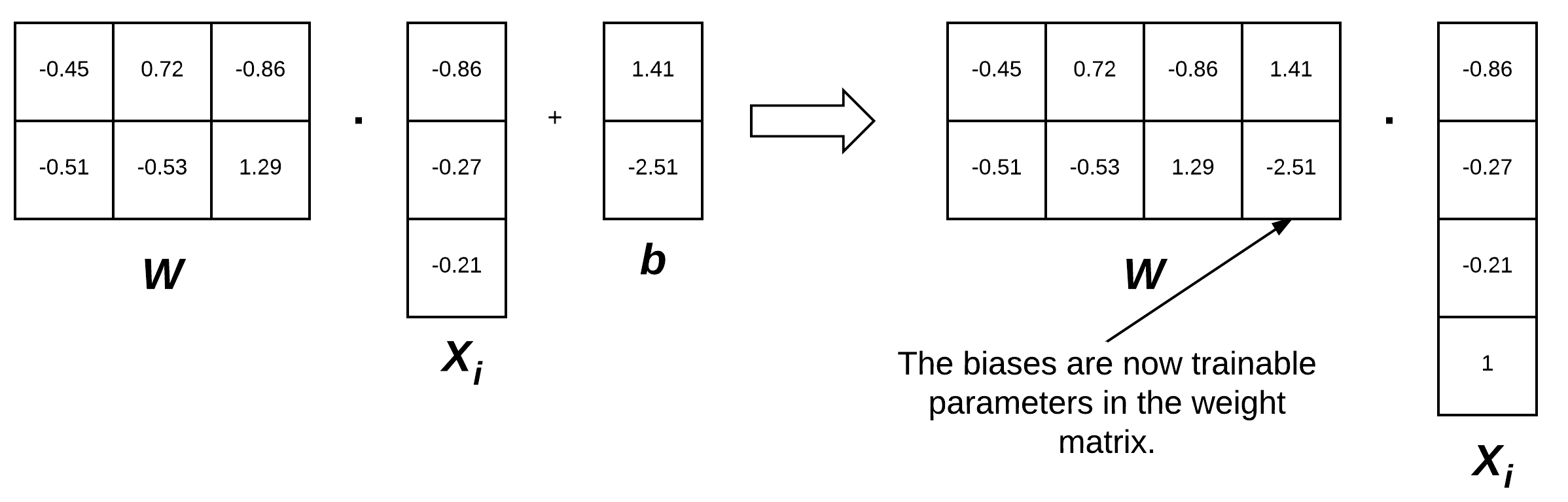
Before we move on to implementing gradient descent, I want to take the time to discuss a technique called the “bias trick,” a method of combining our weight matrix W and bias vector b into a single parameter. Recall from our previous decisions that our scoring function is defined as:

(2)

It’s often tedious to keep track of two separate variables, both in terms of explanation and implementation — to avoid this situation entirely, we can combine W and b together. To combine both the bias and weight matrix, we add an extra dimension (i.e., column) to our input data X that holds a constant 1 — this is our bias dimension.

Typically we either append the new dimension to each individual x_i as the first dimension or the last dimension. In reality, it doesn’t matter. We can choose any arbitrary location to insert a column of ones into our design matrix, as long as it exists. Doing so allows us to rewrite our scoring function via a single matrix multiply:

(3)

Again, we are allowed to omit the b term here as it is embedded into our weight matrix.

In the context of our previous examples in the “Animals” dataset, we’ve worked with 32×32×3 images with a total of 3,072 pixels. Each x_i is represented by a vector of [3072×1]. Adding in a dimension with a constant value of one now expands the vector to be [3073×1]. Similarly, combining both the bias and weight matrix also expands our weight matrix W to be [3×3073] rather than [3×3072]. In this way, we can treat the bias as a learnable parameter within the weight matrix that we don’t have to explicitly keep track of in a separate variable.

To visualize the bias trick, consider Figure 3 (left) where we separate the weight matrix and bias. Up until now, this figure depicts how we have thought of our scoring function. But instead, we can combine the W and b together, provided that we insert a new column into every x_i where every entry is one (Figure 3, right). Applying the bias trick allows us to learn only a single matrix of weights, hence why we tend to prefer this method for implementation. For all future examples, whenever I mention W, assume that the bias vector b is implicitly included in the weight matrix as well.

Remark: We are actually inserting a new row in our feature vector in Figure 3 with a value of 1. You could also add a column to our feature matrix filled with ones. So, which is correct? It actually depends on how you perform your linear algebra and how you are transposing each matrix. You will see both used in the implementation and I want to ensure you are prepared for that now.

Pseudocode for Gradient Descent

Below I have included Python-like pseudocode for the standard, vanilla gradient descent algorithm (pseudocode inspired by cs231n slides):

while True:
	Wgradient = evaluate_gradient(loss, data, W)
	W += -alpha * Wgradient

This pseudocode is what all variations of gradient descent are built off of. We start on Line 1 by looping until some condition is met, typically either:

1. A specified number of epochs has passed (meaning our learning algorithm has “seen” each of the training data points N times).
2. Our loss has become sufficiently low or training accuracy satisfactory high.
3. Loss has not improved in M subsequent epochs.

Line 2 then calls a function named evaluate_gradient. This function requires three parameters:

1. loss: A function used to compute the loss over our current parameters W and input data.
2. data: Our training data where each training sample is represented by an image (or feature vector).
3. W: Our actual weight matrix that we are optimizing over. Our goal is to apply gradient descent to find a W that yields minimal loss.

The evaluate_gradient function returns a vector that is K-dimensional, where K is the number of dimensions in our image/feature vector. The Wgradient variable is the actual gradient, where we have a gradient entry for each dimension.

We then apply gradient descent on Line 3. We multiply our Wgradient by alpha (α), which is our learning rate. The learning rate controls the size of our step.

In practice, you’ll spend a lot of time finding an optimal value of α — it is by far the most important parameter in your model. If α is too large, you’ll spend all of your time bouncing around the loss landscape, never actually “descending” to the bottom of the basin (unless your random bouncing takes you there by pure luck). Conversely, if α is too small, then it will take many (perhaps prohibitively many) iterations to reach the bottom of the basin. Finding the optimal value of α will cause you many headaches — and you’ll spend a considerable amount of your time trying to find an optimal value for this variable for your model and dataset.

Implementing Basic Gradient Descent in Python

Now that we know the basics of gradient descent, let’s implement it in Python and use it to classify some data. Open a new file, name it gradient_descent.py, and insert the following code:

# import the necessary packages
from sklearn.model_selection import train_test_split
from sklearn.metrics import classification_report
from sklearn.datasets import make_blobs
import matplotlib.pyplot as plt
import numpy as np
import argparse

def sigmoid_activation(x):
	# compute the sigmoid activation value for a given input
	return 1.0 / (1 + np.exp(-x))

def sigmoid_deriv(x):
	# compute the derivative of the sigmoid function ASSUMING
	# that the input `x` has already been passed through the sigmoid
	# activation function
	return x * (1 - x)

Lines 2-7 import our required Python packages. We have seen all of these imports before, with the exception of make_blobs, a function used to create “blobs” of normally distributed data points — this is a handy function when testing or implementing our own models from scratch.

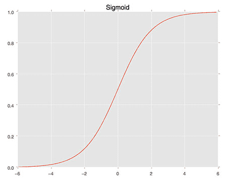
We then define the sigmoid_activation function on Line 9. When plotted this function will resemble an “S”-shaped curve (Figure 4). We call it an activation function because the function will “activate” and fire “ON” (output value > 0.5) or “OFF” (output value <= 0.5) based on the inputs x.

Lines 13-17 define the derivative of the sigmoid function. We need to compute the derivative of this function to derive the actual gradient. The gradient is what enables us to travel down the slope of the optimization surface. We’ll be covering this in more detail in a separate lesson.

The predict function applies our sigmoid activation function and then thresholds it based on whether the neuron is firing (1) or not (0):

def predict(X, W):
	# take the dot product between our features and weight matrix
	preds = sigmoid_activation(X.dot(W))

	# apply a step function to threshold the outputs to binary
	# class labels
	preds[preds <= 0.5] = 0
	preds[preds > 0] = 1

	# return the predictions
	return preds

Given a set of input data points X and weights W, we call the sigmoid_activation function on them to obtain a set of predictions (Line 21). We then threshold the predictions: any prediction with a value <= 0.5 is set to 0 while any prediction with a value > 0.5 is set to 1 (Lines 25 and 26). The predictions are then returned to the calling function on Line 29.

While there are other (better) alternatives to the sigmoid activation function, it makes for an excellent starting point in our discussion of neural networks, deep learning, and gradient-based optimization. I’ll be discussing other activation functions in a future lesson, but for the time being, simply keep in mind that the sigmoid is a non-linear activation function that we can use to threshold our predictions.

Next, let’s parse our command line arguments:

 # construct the argument parse and parse the arguments
ap = argparse.ArgumentParser()
ap.add_argument("-e", "--epochs", type=float, default=100,
	help="# of epochs")
ap.add_argument("-a", "--alpha", type=float, default=0.01,
	help="learning rate")
args = vars(ap.parse_args())

We can provide two (optional) command line arguments to our script:

• --epochs: The number of epochs that we’ll use when training our classifier using gradient descent.
• --alpha: The learning rate for the gradient descent. We typically see 0.1, 0.01, and 0.001 as initial learning rate values, but again, this is a hyperparameter you’ll need to tune for your own classification problems.

Now that our command line arguments are parsed, let’s generate some data to classify:

# generate a 2-class classification problem with 1,000 data points,
# where each data point is a 2D feature vector
(X, y) = make_blobs(n_samples=1000, n_features=2, centers=2,
	cluster_std=1.5, random_state=1)
y = y.reshape((y.shape[0], 1))

# insert a column of 1's as the last entry in the feature
# matrix -- this little trick allows us to treat the bias
# as a trainable parameter within the weight matrix
X = np.c_[X, np.ones((X.shape[0]))]

# partition the data into training and testing splits using 50% of
# the data for training and the remaining 50% for testing
(trainX, testX, trainY, testY) = train_test_split(X, y,
	test_size=0.5, random_state=42)

On Line 41, we make a call to make_blobs, which generates 1,000 data points separated into two classes. These data points are 2D, implying that the “feature vectors” are of length 2. The labels for each of these data points are either 0 or 1. Our goal is to train a classifier that correctly predicts the class label for each data point.

Line 48 applies the “bias trick” (detailed above) that allows us to skip explicitly keeping track of our bias vector b, by inserting a brand new column of 1s as the last entry in our design matrix X. Adding a column containing a constant value across all feature vectors allows us to treat our bias as a trainable parameter within the weight matrix W rather than as an entirely separate variable.

Once we have inserted the column of ones, we partition the data into our training and testing splits on Lines 52 and 53, using 50% of the data for training and 50% for testing.

Our next code block handles randomly initializing our weight matrix using a uniform distribution such that it has the same number of dimensions as our input features (including the bias):

# initialize our weight matrix and list of losses
print("[INFO] training...")
W = np.random.randn(X.shape[1], 1)
losses = []

You might also see both zero and one weight initialization, but as we’ll find out later in our lessons, good initialization is critical to training a neural network in a reasonable amount of time, so random initialization along with simple heuristics win out in the vast majority of circumstances (Mishkin and Matas, 2016).

Line 58 initializes a list to keep track of our losses after each epoch. At the end of your Python script, we’ll plot the loss (which should ideally decrease over time).

All of our variables are now initialized, so we can move on to the actual training and gradient descent procedure:

# loop over the desired number of epochs
for epoch in np.arange(0, args["epochs"]):
	# take the dot product between our features "X" and the weight
	# matrix "W", then pass this value through our sigmoid activation
	# function, thereby giving us our predictions on the dataset
	preds = sigmoid_activation(trainX.dot(W))

	# now that we have our predictions, we need to determine the
	# "error", which is the difference between our predictions and
	# the true values
	error = preds - trainY
	loss = np.sum(error ** 2)
	losses.append(loss)

On Line 61, we start looping over the supplied number of --epochs. By default, we’ll allow the training procedure to “see” each of the training points a total of 100 times (thus, 100 epochs).

Line 65 takes the dot product between our entire training set trainX and our weight matrix W. The output of this dot product is fed through the sigmoid activation function, yielding our predictions.

Given our predictions, the next step is to determine the “error” of the predictions, or more simply, the difference between our predictions and the true values (Line 70). Line 71 computes the least squares error over our predictions, a simple loss typically used for binary classification problems. The goal of this training procedure is to minimize our least squares error. We append this loss to our losses list on Line 72, so we can later plot the loss over time.

Now that we have our error, we can compute the gradient and then use it to update our weight matrix W:

	# the gradient descent update is the dot product between our
	# (1) features and (2) the error of the sigmoid derivative of
	# our predictions
	d = error * sigmoid_deriv(preds)
	gradient = trainX.T.dot(d)

	# in the update stage, all we need to do is "nudge" the weight
	# matrix in the negative direction of the gradient (hence the
	# term "gradient descent" by taking a small step towards a set
	# of "more optimal" parameters
	W += -args["alpha"] * gradient

	# check to see if an update should be displayed
	if epoch == 0 or (epoch + 1) % 5 == 0:
		print("[INFO] epoch={}, loss={:.7f}".format(int(epoch + 1),
			loss))

Lines 77 and 78 handle computing the gradient, which is the dot product between our data points and the error multiplied by the sigmoid derivative of our predictions.

Line 84 is the most critical step in our algorithm and where the actual gradient descent takes place. Here we update our weight matrix W by taking a step in the negative direction of the gradient, thereby allowing us to move toward the bottom of the basin of the loss landscape (hence, the term, gradient descent). After updating our weight matrix, we check to see if an update should be displayed to our terminal (Lines 87-89) and then keep looping until the desired number of epochs has been met — gradient descent is thus an iterative algorithm.

Our classifier is now trained. The next step is evaluation:

# evaluate our model
print("[INFO] evaluating...")
preds = predict(testX, W)
print(classification_report(testY, preds))

To actually make predictions using our weight matrix W, we call the predict method on testX and W on Line 93. Given the predictions, we display a nicely formatted classification report to our terminal on Line 94.

Our last code block handles plotting (1) the testing data so we can visualize the dataset we are trying to classify and (2) our loss over time:

# plot the (testing) classification data
plt.style.use("ggplot")
plt.figure()
plt.title("Data")
plt.scatter(testX[:, 0], testX[:, 1], marker="o", c=testY[:, 0], s=30)

# construct a figure that plots the loss over time
plt.style.use("ggplot")
plt.figure()
plt.plot(np.arange(0, args["epochs"]), losses)
plt.title("Training Loss")
plt.xlabel("Epoch #")
plt.ylabel("Loss")
plt.show()

Simple Gradient Descent Results

To execute our script, simply issue the following command:

$ python gradient_descent.py 
[INFO] training...
[INFO] epoch=1, loss=194.3629849
[INFO] epoch=5, loss=9.3225755
[INFO] epoch=10, loss=5.2176352
[INFO] epoch=15, loss=3.0483912
[INFO] epoch=20, loss=1.8903512
[INFO] epoch=25, loss=1.3532867
[INFO] epoch=30, loss=1.0746259
[INFO] epoch=35, loss=0.9074719
[INFO] epoch=40, loss=0.7956885
[INFO] epoch=45, loss=0.7152976
[INFO] epoch=50, loss=0.6547454
[INFO] epoch=55, loss=0.6078759
[INFO] epoch=60, loss=0.5711027
[INFO] epoch=65, loss=0.5421195
[INFO] epoch=70, loss=0.5192554
[INFO] epoch=75, loss=0.5011559
[INFO] epoch=80, loss=0.4866579
[INFO] epoch=85, loss=0.4747733
[INFO] epoch=90, loss=0.4647116
[INFO] epoch=95, loss=0.4558868
[INFO] epoch=100, loss=0.4478966

As we can see from Figure 5 (left), our dataset is clearly linear separable (i.e., we can draw a line that separates the two classes of data). Our loss also drops dramatically, starting out very high and then quickly dropping (right). We can see just how quickly the loss drops by investigating the terminal output above. Notice how the loss is initially > 194 but drops to ≈ 0.6 by epoch 50. By the time training terminates by epoch 100, our loss has to 0.45.

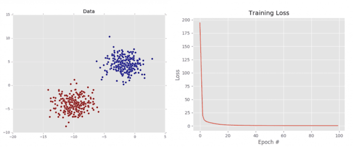
This plot validates that our weight matrix is being updated in a manner that allows the classifier to learn from the training data. We can see the classification report for our dataset below:

[INFO] evaluating...
             precision    recall  f1-score   support

          0       1.00      1.00      1.00       250
          1       1.00      1.00      1.00       250

avg / total       1.00      1.00      1.00       500

Notice how both classes are correctly classified 100% of the time, again, implying that our dataset is both: (1) linearly separable and (2) our gradient descent algorithm was able to descend into an area of low loss, capable of separating the two classes.

That said, it’s important to keep in mind how the vanilla gradient descent algorithm works. Vanilla gradient descent only performs a weight update once for every epoch — in this example, we trained our model for 100 epochs, so only 100 updates took place. Depending on the initialization of the weight matrix and the size of the learning rate, it’s possible that we may not be able to learn a model that can separate the points (even though they are linearly separable).

For simple gradient descent, you are better off training for more epochs with a smaller learning rate to help overcome this issue. However, a variant of gradient descent called Stochastic Gradient Descent performs a weight update for every batch of training data, implying there are multiple weight updates per epoch. This approach leads to a faster, more stable convergence.