Keras Learning Rate Finder

In this tutorial, you will learn how to automatically find learning rates using Keras. This guide provides a Keras implementation of fast.ai’s popular “lr_find” method.

Today is part three in our three-part series of learning rate schedules, policies, and decay using Keras:

1. Part #1: Keras learning rate schedules and decay
2. Part #2: Cyclical Learning Rates with Keras and Deep Learning (last week’s post)
3. Part #3: Keras Learning Rate Finder (today’s post)

Last week we discussed Cyclical Learning Rates (CLRs) and how they can be used to obtain high accuracy models with fewer experiments and limited hyperparameter tuning.

The CLR method allows our learning rate to cyclically oscillate between a lower and upper bound; however, the question still remains, how do we know what are good choices for our learning rates?

Today I’ll be answering that question.

And by the time you have completed this tutorial, you will understand how to automatically find optimal learning rates for your neural network, saving you 10s, 100s or even 1000s of hours in compute time running experiments to tune your hyperparameters.

To learn how to find optimal learning rates using Keras, just keep reading!

Keras Learning Rate Finder

2020-06-11 Update: This blog post is now TensorFlow 2+ compatible!

In the first part of this tutorial, we’ll briefly discuss a simple, yet elegant, algorithm that can be used to automatically find optimal learning rates for your deep neural network.

From there, I’ll show you how to implement this method using the Keras deep learning framework.

We’ll apply the learning rate finder implementation to an example dataset, enabling us to obtain our optimal learning rates.

We’ll then take the found learning rates and fully train our network using a Cyclical Learning Rate policy.

How to automatically find optimal learning rates for your neural network architecture

In last week’s tutorial on Cyclical Learning Rates (CLRs), we discussed Leslie Smith’s 2017 paper, Cyclical Learning Rates for Training Neural Networks.

Based on the title of the paper alone, the obvious contribution to the deep learning community by Dr. Smith is the Cyclical Learning Rate algorithm.

However, there is a second contribution that is arguably more important than CLRs — automatically finding learning rates. Inside the paper, Dr. Smith proposes a simple, yet elegant solution on how we can automatically find optimal learning rates for training.

Note: While the algorithm was introduced by Dr. Smith, it wasn’t popularized until Jermey Howard of fast.ai suggested that his students use it. If you’re a fast.ai user, you may remember the learn.lr_find function — we’ll be implementing a similar method using TensorFlow/Keras instead.

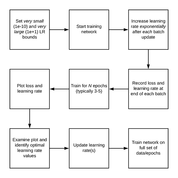
The automatic learning rate finder algorithm works like this:

• Step #1: We start by defining an upper and lower bound on our learning rate. The lower bound should be very small (1e-10) and the upper bound should be very large (1e+1).
  • At 1e-10 the learning rate will be too small for our network to learn, while at 1e+1 the learning rate will be too large and our model will overfit.
  • Both of these are okay, and in fact, that’s what we hope to see!
• Step #2: We then start training our network, starting at the lower bound.
  • After each batch update, we exponentially increase our learning rate.
  • We log the loss after each batch update as well.
• Step #3: Training continues, and therefore the learning rate continues to increase until we hit our maximum learning rate value.
  • Typically, this entire training process/learning rate increase only takes 1-5 epochs.
• Step #4: After training is complete we plot a smoothed loss over time, enabling us to see when the learning rate is both:
  • Just large enough for loss to decrease
  • And too large, to the point where loss starts to increase.

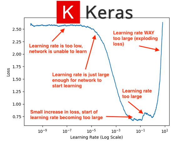
The following figure (which is the same as the header at the very top of the post, but included here again so you can easily follow along) visualizes the output of the learning rate finder algorithm on the CIFAR-10 dataset using a variation of GoogLeNet (which we’ll utilize later in this tutorial):

While examining this plot, keep in mind that our learning rate is exponentially increasing after each batch update. After a given batch completes, we increase the learning rate for the next batch.

Notice that from 1e-10 to 1e-6 our loss is essentially flat — the learning rate is too small for the network to actually learn anything. Starting at approximately 1e-5 our loss starts to decline — this is the smallest learning rate where our network can actually learn.

By the time we hit 1e-4 our network is learning very quickly. At a little past 1e-2 there is a small increase in loss, but the big increase doesn’t begin until 1e-1.

Finally, by 1e+1 our loss has exploded — the learning rate is far too high for our model to learn.

Given this plot, I can visually examine it and pick out my lower and upper bounds on my learning rate for CLR:

• Lower bound: 1e-5
• Upper bound: 1e-2

If you are using a learning rate schedule/decay policy then you would select 1e-2 as your initial learning rate and then decrease it as you train.

However, in this tutorial we’ll be using a Cyclical Learning Rate policy so we need both the lower and upper bound.

But, the question still remains:

How did I generate that learning rate plot?

I’ll be answering that question later in this tutorial.

Configuring your development environment

To configure your system for this tutorial, I first recommend following either of these tutorials:

• How to install TensorFlow 2.0 on Ubuntu
• How to install TensorFlow 2.0 on macOS

Either tutorial will help you configure you system with all the necessary software for this blog post in a convenient Python virtual environment.

Please note that PyImageSearch does not recommend or support Windows for CV/DL projects.

Project structure

Go ahead and grab the “Downloads” for today’s post which contain last week’s CLR implementation and this week’s Learning Rate Finder in addition to our training script.

Then, inspect the project layout with the tree command:

$ tree --dirsfirst
.
├── output
│   ├── clr_plot.png
│   ├── lrfind_plot.png
│   └── training_plot.png
├── pyimagesearch
│   ├── __init__.py
│   ├── clr_callback.py
│   ├── config.py
│   ├── learningratefinder.py
│   └── minigooglenet.py
└── train.py

2 directories, 9 files

Our output/ directory contains three plots:

• The Cyclical Learning Rate graph.
• The Learning Rate Finder loss vs. learning rate plot.
• Our training accuracy/loss history plot.

The pyimagesearch module contains three classes and a configuration:

• clr_callback.py : Contains the CyclicLR class which is implemented as a Keras callback.
• learningratefinder.py : Holds the LearningRateFinder class — the focus of today’s tutorial.
• minigooglenet.py : Has our MiniGoogLeNet CNN class. We won’t go into details today. Please refer to Deep Learning for Computer Vision with Python for a deep dive into GoogLeNet as well as MiniGoogLeNet.
• config.py : A Python file which holds configuration parameters/variables.

After we review the config.py and learningratefinder.py files, we’ll walk through train.py , our Keras CNN training script.

Implementing our automatic Keras learning rate finder

Let’s now define a class named LearningRateFinder that encapsulates the algorithm logic from the “How to automatically find optimal learning rates for your neural network architecture” section above.

Our implementation is inspired by the LRFinder class from the ktrain library — my primary contribution is a few adjustments to the algorithm, including detailed documentation and comments for the source code, making it easier for readers to understand how the algorithm works.

Let’s go ahead and get started — open up the learningratefinder.py file in your project directory and insert the following code:

# import the necessary packages
from tensorflow.keras.callbacks import LambdaCallback
from tensorflow.keras import backend as K
import matplotlib.pyplot as plt
import numpy as np
import tempfile

class LearningRateFinder:
	def __init__(self, model, stopFactor=4, beta=0.98):
		# store the model, stop factor, and beta value (for computing
		# a smoothed, average loss)
		self.model = model
		self.stopFactor = stopFactor
		self.beta = beta

		# initialize our list of learning rates and losses,
		# respectively
		self.lrs = []
		self.losses = []

		# initialize our learning rate multiplier, average loss, best
		# loss found thus far, current batch number, and weights file
		self.lrMult = 1
		self.avgLoss = 0
		self.bestLoss = 1e9
		self.batchNum = 0
		self.weightsFile = None

Packages are imported on Lines 2-6. We’ll use a LambdaCallback to instruct our callback to run at the end of each batch update. We will use matplotlib to implement a method called plot_loss which plots the loss vs. learning rate.

The constructor to the LearningRateFinder class begins on Line 9.

First, we store the initialized model, stopFactor which indicates when to bail out of training (if our loss becomes too large), and beta value (used for averaging/smoothing our loss for visualization purposes).

We then initialize our lists of learning rates along with the loss values for the respective learning rates (Lines 17 and 18).

We proceed to perform a few more initializations, including:

• lrMult: The learning rate multiplication factor.
• avgLoss: Average loss over time.
• bestLoss: The best loss we have found when training.
• batchNum: The current batch number update.
• weightsFile: Our path to the initial model weights (so we can reload the weights and set them to their initial values prior to training after our learning rate has been found).

The reset method is a convenience/helper function used to reset all variables from our constructor:

	def reset(self):
		# re-initialize all variables from our constructor
		self.lrs = []
		self.losses = []
		self.lrMult = 1
		self.avgLoss = 0
		self.bestLoss = 1e9
		self.batchNum = 0
		self.weightsFile = None

When using our LearningRateFinder class, must be able to work with both:

• Data that can fit into memory.
• Data that either (1) is loaded via a data generator and is therefore too large to fit into memory or (2) needs data augmentation/additional processing applied to it and thus uses a generator.

If the entire dataset can fit into memory and no data augmentation is applied, we can use Keras’ .fit method to train our model.

However, if we are using a data generator, either out of memory necessity or because we are applying data augmentation, we instead need to use Keras’ .fit function with an Image Data Generator object as the first argument for training.

Note: You can read about the differences between .fit and .fit_generator in this tutorial. Note that .fit_generator function is deprecated and .fit is capable of data augmentation now.

The is_data_generator function can determine if our input data is a raw NumPy array or if we are using a data generator:

	def is_data_iter(self, data):
		# define the set of class types we will check for
		iterClasses = ["NumpyArrayIterator", "DirectoryIterator",
			 "DataFrameIterator", "Iterator", "Sequence"]

		# return whether our data is an iterator
		return data.__class__.__name__ in iterClasses

Here we are checking to see if the name of the input data class belongs to the set of data iterator classes defined in Lines 41 and 42.

If you are using your own custom data generator simply encapsulate it in a class and then add your class name to the list of iterClasses.

The on_batch_end function is responsible for updating our learning rate after every batch is complete (i.e., both the forward and backward pass):

	def on_batch_end(self, batch, logs):
		# grab the current learning rate and add log it to the list of
		# learning rates that we've tried
		lr = K.get_value(self.model.optimizer.lr)
		self.lrs.append(lr)

		# grab the loss at the end of this batch, increment the total
		# number of batches processed, compute the average average
		# loss, smooth it, and update the losses list with the
		# smoothed value
		l = logs["loss"]
		self.batchNum += 1
		self.avgLoss = (self.beta * self.avgLoss) + ((1 - self.beta) * l)
		smooth = self.avgLoss / (1 - (self.beta ** self.batchNum))
		self.losses.append(smooth)

		# compute the maximum loss stopping factor value
		stopLoss = self.stopFactor * self.bestLoss

		# check to see whether the loss has grown too large
		if self.batchNum > 1 and smooth > stopLoss:
			# stop returning and return from the method
			self.model.stop_training = True
			return

		# check to see if the best loss should be updated
		if self.batchNum == 1 or smooth < self.bestLoss:
			self.bestLoss = smooth

		# increase the learning rate
		lr *= self.lrMult
		K.set_value(self.model.optimizer.lr, lr)

We’ll be using this method as a Keras callback and therefore we need to ensure our function accepts two variables Keras expects to see — batch and logs.

Lines 50 and 51 grab the current learning rate from our optimizer and then add it to our learning rates list (lrs ).

Lines 57 and 58 grab the loss at the end of the batch and then increment our batch number.

Lines 58-61 compute the average loss, smooth it, and then update the losses list with the smooth average.

Line 64 computes our maximum loss value which is a function of our stopFactor and our bestLoss found thus far.

If our smoothLoss has grown to be larger than our stopLoss, then we stop training (Lines 67-70).

Lines 73 and 74 check to see if a new bestLoss has been found, and if so, we update the variable.

Finally, Line 77 increases our learning rate while Line 78 sets the learning rate value for the next batch.

Our next method, find, is responsible for automatically finding our optimal learning rate for training. We’ll call this method from our driver script when we are ready to find our learning rate:

	def find(self, trainData, startLR, endLR, epochs=None,
		stepsPerEpoch=None, batchSize=32, sampleSize=2048,
		verbose=1):
		# reset our class-specific variables
		self.reset()

		# determine if we are using a data generator or not
		useGen = self.is_data_iter(trainData)

		# if we're using a generator and the steps per epoch is not
		# supplied, raise an error
		if useGen and stepsPerEpoch is None:
			msg = "Using generator without supplying stepsPerEpoch"
			raise Exception(msg)

		# if we're not using a generator then our entire dataset must
		# already be in memory
		elif not useGen:
			# grab the number of samples in the training data and
			# then derive the number of steps per epoch
			numSamples = len(trainData[0])
			stepsPerEpoch = np.ceil(numSamples / float(batchSize))

		# if no number of training epochs are supplied, compute the
		# training epochs based on a default sample size
		if epochs is None:
			epochs = int(np.ceil(sampleSize / float(stepsPerEpoch)))

Our find method accepts a number of parameters, including:

• trainData: Our training data (either a NumPy array of data or a data generator).
• startLR: The initial, starting learning rate.
• epochs: The number of epochs to train for (if no value is supplied we’ll compute the number of epochs).
• stepsPerEpoch: The total number of batch update steps per each epoch.
• batchSize: The batch size of our optimizer.
• sampleSize: The number of samples from trainData to use when finding the optimal learning rate.
• verbose: Verbosity setting for Keras’ .fit method.

Line 84 resets our class-specific variables while Line 87 checks to see if we are using a data iterator or a raw NumPy array.

In the case that we are using a data generator and there is no stepsPerEpoch variable supplied, we raise an exception since we cannot possibly determine the stepsPerEpoch from a generator (see this tutorial for more information on why this is true).

Otherwise, if we are not using a data generator we grab the numSamples from the trainData and then compute the number of stepsPerEpoch by dividing the number of data points by our batchSize (Lines 97-101).

Finally, if no number of epochs were supplied, we compute the number of training epochs by dividing the sampleSize by the number of stepsPerEpoch. My personal preference is to have the number of epochs ultimately be in the 3-5 range — long enough to obtain reliable results but not so long that I waste hours and hours of training time.

Let’s move on to the heart of the automatic learning rate finder algorithm:

		# compute the total number of batch updates that will take
		# place while we are attempting to find a good starting
		# learning rate
		numBatchUpdates = epochs * stepsPerEpoch

		# derive the learning rate multiplier based on the ending
		# learning rate, starting learning rate, and total number of
		# batch updates
		self.lrMult = (endLR / startLR) ** (1.0 / numBatchUpdates)

		# create a temporary file path for the model weights and
		# then save the weights (so we can reset the weights when we
		# are done)
		self.weightsFile = tempfile.mkstemp()[1]
		self.model.save_weights(self.weightsFile)

		# grab the *original* learning rate (so we can reset it
		# later), and then set the *starting* learning rate
		origLR = K.get_value(self.model.optimizer.lr)
		K.set_value(self.model.optimizer.lr, startLR)

Line 111 computes the total number of batch updates that will take place when finding our learning rate.

Using the numBatchUpdates we deriving the learning rate multiplication factor (lrMult) which is used to exponentially increase our learning rate (Line 116).

Lines 121 and 122 create a temporary file to store our model’s initial weights. We’ll then restore these weights when our learning rate finder has completed running.

Next, we grab the original learning rate for the optimizer (Line 126), store it in origLR , and then instruct Keras to set the initial learning rate (startLR ) for the optimizer.

Let’s create our LambdaCallback which will call our on_batch_end method each time a batch completes:

		# construct a callback that will be called at the end of each
		# batch, enabling us to increase our learning rate as training
		# progresses
		callback = LambdaCallback(on_batch_end=lambda batch, logs:
			self.on_batch_end(batch, logs))

		# check to see if we are using a data iterator
		if useGen:
			self.model.fit(
				x=trainData,
				steps_per_epoch=stepsPerEpoch,
				epochs=epochs,
				verbose=verbose,
				callbacks=[callback])

		# otherwise, our entire training data is already in memory
		else:
			# train our model using Keras' fit method
			self.model.fit(
				x=trainData[0], y=trainData[1],
				batch_size=batchSize,
				epochs=epochs,
				callbacks=[callback],
				verbose=verbose)

		# restore the original model weights and learning rate
		self.model.load_weights(self.weightsFile)
		K.set_value(self.model.optimizer.lr, origLR)

Lines 132 and 133 construct our callback — each time a batch completes the on_batch_end method will be called to automatically update our learning rate.

In the event we’re using a data generator, we’ll train our model using the .fit_generator method (Lines 136-142). Otherwise, our entire training data exists in memory as a NumPy array, so we can use the .fit method (Lines 145- 152).

After training is complete, we reset the initial model weights and learning rate value (Lines 155 and 156).

Our final method, plot_loss, is used to plot both our learning rates and losses over time:

	def plot_loss(self, skipBegin=10, skipEnd=1, title=""):
		# grab the learning rate and losses values to plot
		lrs = self.lrs[skipBegin:-skipEnd]
		losses = self.losses[skipBegin:-skipEnd]

		# plot the learning rate vs. loss
		plt.plot(lrs, losses)
		plt.xscale("log")
		plt.xlabel("Learning Rate (Log Scale)")
		plt.ylabel("Loss")

		# if the title is not empty, add it to the plot
		if title != "":
			plt.title(title)

This exact method generated the plot you saw in Figure 2.

Later, in the “Finding our optimal learning rate with Keras” section of this tutorial, you’ll discover how to use the LearningRateFinder class we just implemented to automatically find optimal learning rates with Keras.

Our configuration file

Before we implement our actual training script, let’s create our configuration.

Open up the config.py file and insert the following code:

# import the necessary packages
import os

# initialize the list of class label names
CLASSES = ["top", "trouser", "pullover", "dress", "coat",
	"sandal", "shirt", "sneaker", "bag", "ankle boot"]

# define the minimum learning rate, maximum learning rate, batch size,
# step size, CLR method, and number of epochs
MIN_LR = 1e-5
MAX_LR = 1e-2
BATCH_SIZE = 64
STEP_SIZE = 8
CLR_METHOD = "triangular"
NUM_EPOCHS = 48

# define the path to the output learning rate finder plot, training
# history plot and cyclical learning rate plot
LRFIND_PLOT_PATH = os.path.sep.join(["output", "lrfind_plot.png"])
TRAINING_PLOT_PATH = os.path.sep.join(["output", "training_plot.png"])
CLR_PLOT_PATH = os.path.sep.join(["output", "clr_plot.png"])

We’ll be using the Fashion MNIST as the dataset for this project. Lines 5 and 6 set the class labels for the Fashion MNIST dataset.

Our Cyclical Learning Rate parameters are specified on Lines 10-15. The MIN_LR and MAX_LR will be found in the “Finding our optimal learning rate with Keras” section below, but we’re including them here as a matter of completeness. If you need to review these parameters, please refer to last week’s post.

We will output three types of plots and the paths are specified via Lines 19-21. Two of the plots will be the same format as last week’s (training and CLR). The new type is the “learning rate finder” plot.

Implementing our learning rate finder training script

Our learning rate finder script will be responsible for both:

1. Automatically finding our initial learning rate using the LearningRateFinder class we implemented earlier in this guide
2. And taking the learning rate values we find and then training the network on the entire dataset.

Let’s go ahead and get started!

Open up the train.py file and insert the following code:

# set the matplotlib backend so figures can be saved in the background
import matplotlib
matplotlib.use("Agg")

# import the necessary packages
from pyimagesearch.learningratefinder import LearningRateFinder
from pyimagesearch.minigooglenet import MiniGoogLeNet
from pyimagesearch.clr_callback import CyclicLR
from pyimagesearch import config
from sklearn.preprocessing import LabelBinarizer
from sklearn.metrics import classification_report
from tensorflow.keras.preprocessing.image import ImageDataGenerator
from tensorflow.keras.optimizers import SGD
from tensorflow.keras.datasets import fashion_mnist
import matplotlib.pyplot as plt
import numpy as np
import argparse
import cv2
import sys

Lines 2-19 import our required packages. Notice how we import our LearningRateFinder as well as our CyclicLR callback. We’ll be training MiniGoogLeNet on fashion_mnist . To learn more about the dataset, be sure to read Fashion MNIST with Keras and Deep Learning.

Let’s go ahead and parse a command line argument:

# construct the argument parser and parse the arguments
ap = argparse.ArgumentParser()
ap.add_argument("-f", "--lr-find", type=int, default=0,
	help="whether or not to find optimal learning rate")
args = vars(ap.parse_args())

We have a single command line argument, --lr-find , a flag which indicates whether or not to find the optimal learning rate.

Next, let’s prepare our data:

# load the training and testing data
print("[INFO] loading Fashion MNIST data...")
((trainX, trainY), (testX, testY)) = fashion_mnist.load_data()

# Fashion MNIST images are 28x28 but the network we will be training
# is expecting 32x32 images
trainX = np.array([cv2.resize(x, (32, 32)) for x in trainX])
testX = np.array([cv2.resize(x, (32, 32)) for x in testX])

# scale the pixel intensities to the range [0, 1]
trainX = trainX.astype("float") / 255.0
testX = testX.astype("float") / 255.0

# reshape the data matrices to include a channel dimension (required
# for training)
trainX = trainX.reshape((trainX.shape[0], 32, 32, 1))
testX = testX.reshape((testX.shape[0], 32, 32, 1))

# convert the labels from integers to vectors
lb = LabelBinarizer()
trainY = lb.fit_transform(trainY)
testY = lb.transform(testY)

# construct the image generator for data augmentation
aug = ImageDataGenerator(width_shift_range=0.1,
	height_shift_range=0.1, horizontal_flip=True,
	fill_mode="nearest")

Here we:

• Load the Fashion MNIST dataset (Line 29).
• Resize each image from 28×28 images to 32×32 images (what our network expects the inputs to be) on Lines 33 and 34.
• Scale pixel intensities to the range [0, 1] (Lines 37 and 38).
• Binarize labels (Lines 46-48).
• Construct our data augmentation object (Lines 51-53). Read more about data augmentation in my previous posts as well as in the Practitioner Bundle of Deep Learning for Computer Vision with Python.

From here, we can compile our model :

# initialize the optimizer and model
print("[INFO] compiling model...")
opt = SGD(lr=config.MIN_LR, momentum=0.9)
model = MiniGoogLeNet.build(width=32, height=32, depth=1, classes=10)
model.compile(loss="categorical_crossentropy", optimizer=opt,
	metrics=["accuracy"])

Our model is compiled with SGD (Stochastic Gradient Descent) optimization. We use "categorical_crossentropy" loss since we have > 2 classes. Be sure to use "binary_crossentropy" if your dataset only has 2 classes.

The following if-then block handles the case when we’re finding the optimal learning rate:

# check to see if we are attempting to find an optimal learning rate
# before training for the full number of epochs
if args["lr_find"] > 0:
	# initialize the learning rate finder and then train with learning
	# rates ranging from 1e-10 to 1e+1
	print("[INFO] finding learning rate...")
	lrf = LearningRateFinder(model)
	lrf.find(
		aug.flow(trainX, trainY, batch_size=config.BATCH_SIZE),
		1e-10, 1e+1,
		stepsPerEpoch=np.ceil((len(trainX) / float(config.BATCH_SIZE))),
		batchSize=config.BATCH_SIZE)

	# plot the loss for the various learning rates and save the
	# resulting plot to disk
	lrf.plot_loss()
	plt.savefig(config.LRFIND_PLOT_PATH)

	# gracefully exit the script so we can adjust our learning rates
	# in the config and then train the network for our full set of
	# epochs
	print("[INFO] learning rate finder complete")
	print("[INFO] examine plot and adjust learning rates before training")
	sys.exit(0)

Line 64 checks to see if we should attempt to find optimal learning rates. Assuming so, we:

• Initialize LearningRateFinder (Line 68).
• Start training with a 1e-10 learning rate and exponentially increase it until we hit 1e+1 (Lines 69-73).
• Plot the loss vs. learning rate and save the resulting figure (Lines 77 and 78).
• Gracefully exit the script after printing a couple of messages to the user (Lines 83-85).

After this code executes we now need to:

1. Review the generated plot.
2. Update config.py with our MIN_LR and MAX_LR, respectively.
3. Train the network on our full dataset.

Assuming we have completed steps 1 and 2, now let’s handle the 3rd step where our minimum and maximum learning rate have already been found and updated in the config. In this case, it is time to initialize our Cyclical Learning Rate class and commence training:

# otherwise, we have already defined a learning rate space to train
# over, so compute the step size and initialize the cyclic learning
# rate method
stepSize = config.STEP_SIZE * (trainX.shape[0] // config.BATCH_SIZE)
clr = CyclicLR(
	mode=config.CLR_METHOD,
	base_lr=config.MIN_LR,
	max_lr=config.MAX_LR,
	step_size=stepSize)

# train the network
print("[INFO] training network...")
H = model.fit(
	x=aug.flow(trainX, trainY, batch_size=config.BATCH_SIZE),
	validation_data=(testX, testY),
	steps_per_epoch=trainX.shape[0] // config.BATCH_SIZE,
	epochs=config.NUM_EPOCHS,
	callbacks=[clr],
	verbose=1)

# evaluate the network and show a classification report
print("[INFO] evaluating network...")
predictions = model.predict(x=testX, batch_size=config.BATCH_SIZE)
print(classification_report(testY.argmax(axis=1),
	predictions.argmax(axis=1), target_names=config.CLASSES))

2020-06-11 Update: Formerly, TensorFlow/Keras required use of a method called .fit_generator in order to accomplish data augmentation. Now, the .fit method can handle data augmentation as well, making for more-consistent code. This also applies to the migration from .predict_generator to .predict. Be sure to check out my articles about fit and fit_generator as well as data augmentation.

Our CyclicLR is initialized with the freshly set parameters in our config file (Lines 90-95).

Then our model is trained using .fit_generator with our aug data augmentation object and our clr callback (Lines 99-105).

Upon training completion, we proceed to evaluate our network on the testing set (Line 109). A classification_report is printed in the terminal for us to inspect.

Finally, let’s plot both our training history and CLR history:

# construct a plot that plots and saves the training history
N = np.arange(0, config.NUM_EPOCHS)
plt.style.use("ggplot")
plt.figure()
plt.plot(N, H.history["loss"], label="train_loss")
plt.plot(N, H.history["val_loss"], label="val_loss")
plt.plot(N, H.history["accuracy"], label="train_acc")
plt.plot(N, H.history["val_accuracy"], label="val_acc")
plt.title("Training Loss and Accuracy")
plt.xlabel("Epoch #")
plt.ylabel("Loss/Accuracy")
plt.legend(loc="lower left")
plt.savefig(config.TRAINING_PLOT_PATH)

# plot the learning rate history
N = np.arange(0, len(clr.history["lr"]))
plt.figure()
plt.plot(N, clr.history["lr"])
plt.title("Cyclical Learning Rate (CLR)")
plt.xlabel("Training Iterations")
plt.ylabel("Learning Rate")
plt.savefig(config.CLR_PLOT_PATH)

2020-06-11 Update: In order for this plotting snippet to be TensorFlow 2+ compatible the H.history dictionary keys are updated to fully spell out “accuracy” sans “acc” (i.e., H.history["val_accuracy"] and H.history["accuracy"]). It is semi-confusing that “val” is not spelled out as “validation”; we have to learn to love and live with the API and always remember that it is a work in progress that many developers around the world contribute to.

Two plots are generated for the training procedure to accompany the learning rate finder plot that we already should have:

• Training accuracy/loss history (Lines 114-125). The standard plot format included in most of my tutorials and every experiment of my deep learning book.
• Learning rate history (Lines 128-134). This plot will help us to visually verify that our learning rate is oscillating according to our CLR intentions.

Finding our optimal learning rate with Keras

We are now ready to find our optimal learning rates!

Make sure you’ve used the “Downloads” section of the tutorial to download the source code — from there, open up a terminal and execute the following command:

$ python train.py --lr-find 1
[INFO] loading Fashion MNIST data...
[INFO] compiling model...
[INFO] finding learning rate...
Epoch 1/3
938/938 [==============================] - 23s 24ms/step - loss: 2.5839 - accuracy: 0.1072
Epoch 2/3
938/938 [==============================] - 21s 23ms/step - loss: 2.1177 - accuracy: 0.2587
Epoch 3/3
938/938 [==============================] - 21s 23ms/step - loss: 1.0178 - accuracy: 0.6591
[INFO] learning rate finder complete
[INFO] examine plot and adjust learning rates before training

The --lr-find flag instructs our script to utilize the LearningRateFinder class to exponentially increase our learning rate from 1e-10 to 1e+1.

The learning rate is increased after each batch update until our max learning rate is achieved.

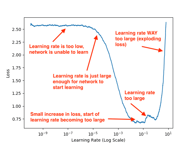
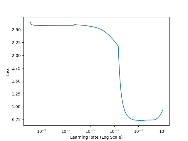
Figure 3 visualizes our loss:

• Loss is stagnant and does not decrease from 1e-10 to approximately 1e-6, implying that the learning rate is too small and our network is not learning.
• At approximately 1e-5 our loss starts to decrease, meaning that our learning rate is just large enough that the model can start to learn.
• By 1e-3 loss is dropping rapidly, indicating that this is a “sweet spot” where the network can learn quickly.
• Just after 1e-1 there is a tiny increase in loss, implying that our learning rate may soon be too large.
• And by the time we reach 1e+1, our loss is beginning to explode (the learning rate is far too large).

Based on this plot, we should choose 1e-5 as our base learning rate and 1e-2 as our max learning rate — these values indicate a learning rate just small enough for our network to start to learn, along with a learning rate that this is large enough for our network to rapidly learn, but not so large that our loss explodes.

Be sure to refer back to Figure 2 if you need help analyzing Figure 3.

Training the entire network architecture

If you haven’t yet, go back to our config.py file and set MIN_LR = 1e-5 and MAX_LR = 1e-2, respectively:

# define the minimum learning rate, maximum learning rate, batch size,
# step size, CLR method, and number of epochs
MIN_LR = 1e-5
MAX_LR = 1e-2
BATCH_SIZE = 64
STEP_SIZE = 8
CLR_METHOD = "triangular"
NUM_EPOCHS = 48

From there, execute the following command:

$ python train.py
[INFO] loading Fashion MNIST data...
[INFO] compiling model...
[INFO] training network...
Epoch 1/48
937/937 [==============================] - 25s 27ms/step - loss: 1.2759 - accuracy: 0.5528 - val_loss: 0.7126 - val_accuracy: 0.7350
Epoch 2/48
937/937 [==============================] - 24s 26ms/step - loss: 0.5589 - accuracy: 0.7946 - val_loss: 0.5217 - val_accuracy: 0.8108
Epoch 3/48
937/937 [==============================] - 25s 26ms/step - loss: 0.4338 - accuracy: 0.8417 - val_loss: 0.5276 - val_accuracy: 0.8017
...
Epoch 46/48
937/937 [==============================] - 25s 26ms/step - loss: 0.0942 - accuracy: 0.9657 - val_loss: 0.1895 - val_accuracy: 0.9379
Epoch 47/48
937/937 [==============================] - 24s 26ms/step - loss: 0.0861 - accuracy: 0.9684 - val_loss: 0.1813 - val_accuracy: 0.9408
Epoch 48/48
937/937 [==============================] - 25s 26ms/step - loss: 0.0791 - accuracy: 0.9714 - val_loss: 0.1741 - val_accuracy: 0.9433
[INFO] evaluating network...
              precision    recall  f1-score   support

         top       0.91      0.89      0.90      1000
     trouser       0.99      0.99      0.99      1000
    pullover       0.92      0.92      0.92      1000
       dress       0.95      0.94      0.94      1000
        coat       0.92      0.93      0.92      1000
      sandal       0.99      0.99      0.99      1000
       shirt       0.82      0.84      0.83      1000
     sneaker       0.97      0.98      0.97      1000
         bag       0.99      1.00      0.99      1000
  ankle boot       0.98      0.97      0.97      1000

    accuracy                           0.94     10000
   macro avg       0.94      0.94      0.94     10000
weighted avg       0.94      0.94      0.94     10000

After training completes we are obtaining 94% accuracy on the Fashion MNIST dataset.

Again, keep in mind that we only ran one experiment to tune the learning rates to our model.

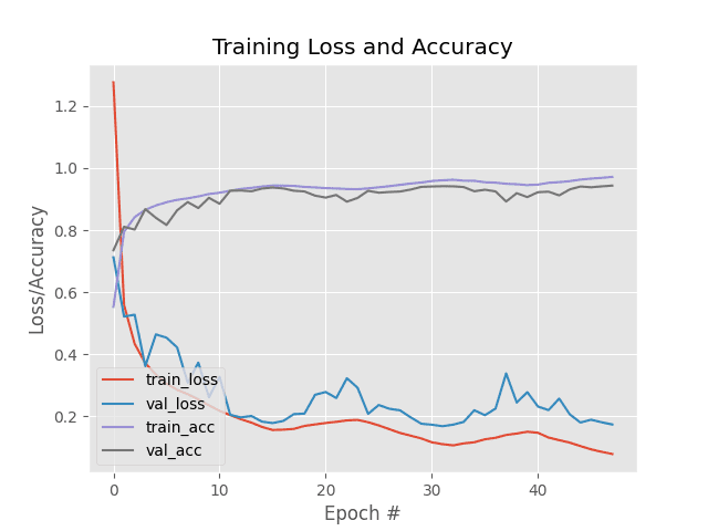
Our training history is plotted in Figure 4. Notice the characteristic “waves” from a triangular Cyclical Learning Rate policy — our training and validation loss gently rides the waves up and down as our learning rate increases and decreases.

Speaking of the Cyclical Learning Rate policy, let’s look at how the learning rate changes during training:

Here we complete three full cycles of the triangular policy, starting at an initial learning rate of 1e-5, increasing to 1e-2, and then decreasing back to 1e-5 again.

Using a combination of Cyclical Learning Rates along with our automatic learning rate finder implementation, we are able to obtain a highly accurate model in only a single experiment!

You can use this combination of CLRs and automatic learning rate finder in your own projects to help you quickly and effectively tune your learning rates.

Summary

In this tutorial you learned how to create an automatic learning rate finder using the Keras deep learning library.

This automatic learning rate finder algorithm follows the suggestions of Dr. Leslie Smith in their 2017 paper, Cyclical Learning Rates for Training Neural Networks (but the method itself wasn’t popularized until Jermey Howard suggested that fast.ai users utilize it).

The primary contribution of this guide is to provide a well-documented Keras learning rate finder, including an example of how to use it.

You can use this learning rate finder implementations when training your own neural networks using Keras, enabling you to:

1. Bypass 10s to 100s of experiments tuning your learning rate.
2. Obtain a high accuracy model with less effort.

Make sure you use this implementation when exploring learning rates with your own datasets and architectures.

I hope you enjoyed my final post in a series of tutorials on finding, tuning, and scheduling learning rates with Keras!

To download the source code to this post (and be notified when future tutorials are published here on PyImageSearch), just enter your email address in the form below!